Lecture 1: Introduction

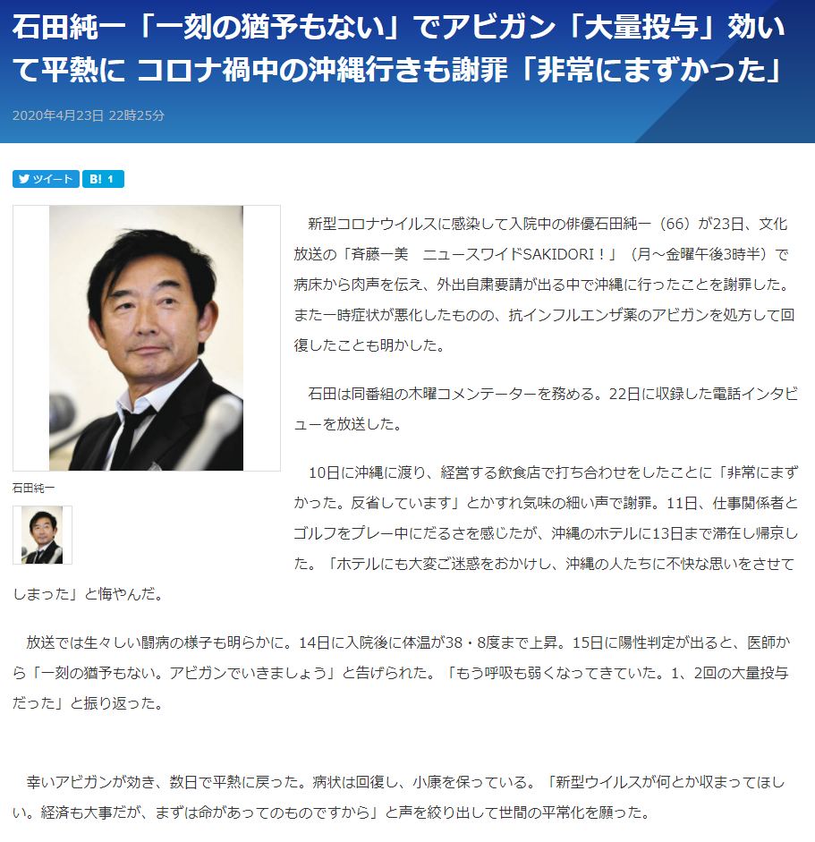
class: center, middle, inverse, title-slide

# Lecture 1: Introduction
### Instructor: Yuta TOYAMA (遠山 祐太)
### Last updated: 2021-06-08

---

class: title-slide-section, center, middle
name: logistics

# Welcome to the Course!!

---

## About me

- Instructor: Yuta Toyama

- Research Field: Industrial Organization, Applied Econometrics, Energy and Environmental Economics

---

## Data analysis is more important than ever

.center[![Data Scientist](figs/DataScientist.png)]

---

## Goal of the Course

- We will learn **causal inference (因果推論) ** in economics.

- Goal 1: How to establish **causality** in data analysis.
    - Various tools: RCT, regression, IV, DID, RD, structural estimation
    - Implementation using R language.
    - **Students who took this course before won an award at the Data Science Competition and the thesis competition.**
  
  
- Goal 2: How to critically examine causal statements in research and journalism.
    - **Is my "causal" claim above really true?**

---

## Contents today

1. What is causality?

2. Case: Data analysis during the Covid-19 crisis

3. Review of Probability: Conditional Expectation

---
class: title-slide-section, center, middle
name: logistics

# What is Causality?

---

## Causal Questions in Economics and Political Science

- Causality (因果): X causes/affects/impacts Y **holding other things fixed *(ceteris paribus)***

- Many questions are causal!
  - How much does an additional year of schooling increase your wage ?
  - How does online advertisement affect sales of products?
  - Do mergers between firms increase product prices?
  - Does democracy cause economic growth?
  - Does higher turnout benefit Democrats in presidential election?

---

## Theoretical Models Implies Causal Relationship

- Consumers' Utility maximization:
    - Higher income leads to more consumption (all else being fixed)
    - Higher price (typically) implies less consumption (all else being fixed)

- Educational investment leads to higher income due to 
    - higher human capital (人的資本)
    - signalling effect (シグナリング)

- Government spending stimulates GDP by multiplier effect (乗数効果)

---

## Data Analysis to Establish Causality

- With data, we want to understand what is going on in reality.

- Ex 1: Test whether theoretical prediction is true.

- Ex 2: Determine the sign of ambiguous theoretical prediction.

---
## Descriptive Analysis (記述統計)

- Describe the data (sample) as a first step.
    - College grads earn 98% more per hour than others
    - Income inequality higher now than 30 years ago
    - Health care costs growing more slowly after the Affordable Care Act (ACA)
    - Airline prices higher now than before merger wave

- Such analysis tells you the **correlation (相関)** between two variables

---

## Does **correlation** imply **causality**?

- Example 1: Cities with many police officers have more crimes (positive correlation).
   - Does this really mean “X (police officers) causes Y (crimes)”?

- Example 2: Those who went to college earn more money by 10%.
  - Is this difference only due to college?

---

## Three possible channels

1. Causality
2. Reverse causality
3. Third factor, or **confounder (交絡因子)**
    - often called **spurious correlation (見せかけの相関)**

---
## Three Channels in Figure

---

## Case: Is Avigan effective treatment for COVID-19?

- Some Japanese celebrities who caught COVID-19 report their own experience that Anti-flu drug Avigan was effective for recovery.
  - [An episode from Junichi Ishida](https://www.chunichi.co.jp/chuspo/article/entertainment/news/CK2020042302100136.html)

- Does this mean Avigan is a silver bullet for COVID-19?

- Why do we care? 
  - Side effects of Avigan, resource allocation of public funds, etc.

---

.center[![Data Scientist](figs/news_avigan.png)]

---

## Difficulty 1: Counterfactual (反実仮想)

- **Counterfactual outcome** is never observed

- Even without Avigan, a patient might have gotten better.

---

## Difficulty 2: Endogenous selection of treatment

- Suppose we have data on patients who got and did not get Avigan in their treatment.

- Does comparison of those people give you treatment effect of Avigan?

- Issue: Those who get Avigan and who do not get might be quite different in other aspects.

---

## Solution: Clinical Trial

- Collect patients and **randomly** choose patients who are given the treatment.
  - Treatment group and control group.

- Compare the outcome of treatment and control group to see the effectiveness of treatment.

- Since 2020, various institutes have been conducting a clinical trial on Avigan for COVID-19. The results have been not assuring, though.

---
class: title-slide-section, center, middle
name: COVID19

# Case: Data Analysis during the COVID-19 Crisis

---

# Data Analysis during the COVID-19 Crisis

- Perhaps, you might have started to see data analysis in the news more often than ever.
    - `#` of positive cases each day
    - flow of people (人流) based on mobile phone location (e.g., Agoop, NTT Docomo)
    - Effective reproduction number (実効再生算数)
    - Efficacy of COVID-19 vaccine from clinical trial

- Researchers in many fields have been conducting various analysis to tackle the crisis.

- Some examples in Economics
    - Macroeconomic analysis using SEIR (Susceptible-Exposed-Infectious-Recovered) model
    - Nowcasting (ナウキャスティング) using alternative data (オルタナティブデータ)
    - Evaluation of various policies towards the crisis. -> more on later

---

# Reference: 経済セミナー別冊「新型コロナ危機に経済学で挑む」

---

# Difficulties in Policy Analysis

- 1: **Observational study (観察研究)**: 
    - Data is observation of what people actually do.
    - Unlike clinical trial, cannot randomize treatment of policy in general.

- 2: Data limitation
    - May not be able to observe what researchers need.

- With these obstacles, we still need to **draw the conclusion while clearly acknowledging its limitations**.

---

# Case: Special Cash Payment

- Special Cash Payment (特別定額給付金): 100,000 JPY for everyone.

- Question: How much did people actually spend?
    
    
- Why we care?
    - Controversial policy (both supporters and )
    - Many countries have done a similar policy.

- Three empirical studies on this issue:
    - Kubota, Onishi, and Toyama (2021): Bank account data
    - Kaneda, Kubota, and Tanaka (2021): Financial app data
    - 宇南山・古村・服部 (2021): Official household survey (「家計調査」)

- I will explain Kubota, Onishi, and Toyama (2021) in detail.

---
class: title-slide-section, center, middle
name: logistics

# Review of Conditional Expectation

---
# Conditional Expectation (条件付き期待値)

- Overview
    - We are interested in the relationship between two different variables, say `$X$` and `$Y$`.
    - Conditional expectation is a way to characterize such relationship
    - Quick review of conditional expectation.

-  Reference
    - Angrist and Pischke MHE Chapter 2 and 3.
    - 奥井ら

---

# Conditional Distribution (条件付き分布)

- Let `$Y$` and `$X$` be the random variables (確率変数). 
    - Let's say `$Y$` is the outcome variable and `$X$` is the explanatory variable.

- The probability distribution function (確率分布関数)
    - Discrete (離散): `$$P(y,x)=Prob(X=x,Y=y)$$` for `$y\in\{y_{1},\cdots,y_{L}\}$` and `$x\in\{x_{1},\cdots,x_{L}\}$`
    - Continuous (連続): the density function (密度関数) `$f(y,x)$` for `$x\in\mathbb{R}$` and `$y\in\mathbb{R}$`.

---

- The conditional probability mass function for discrete case `$$P(y|x)=\frac{P(y,x)}{P(x)}$$` where `$P(x)=\sum_{i=1}^{N}P(y_{i},x)$`

- The conditional density function for continuous case `$f(y|x)=\frac{f(y,x)}{f(x)}$`

---
# Conditional Expectation (条件付き期待値)

- The **conditional expectation** function `$$E[Y|X]=\sum_{l=1}^{L}y_{l}P(Y=y_{l}|X)$$` for a discrete case and `$$E[Y|X]=\int_{-\infty}^{\infty}yf(y|X)dy$$` for a continuous case.

---

## Properties of Conditional Expectation Function

- Proposition CE1 `$$E[c(X)|X]=c(X)$$` for a function `$c(\cdot)$`.

- Proposition CE2 (linearity) `$$E[a(X)Y+b(X)|X]=a(X)E[Y|X]+b(X)$$` for function `$a(\cdot)$` and `$b(\cdot)$`.

- Proposition CE3. If `$X$` and `$Y$` are independent, then `$E[Y|X]=E[Y]$`

---

- Proof of CE3 (for a discrete case):

`\begin{eqnarray}
E[Y|X]&=&\sum_{l=1}^{L}y_{l}P(Y=y_{l}|X) \\
	  &=&\sum_{l=1}^{L}y_{l}\frac{P(Y=y_{l},X)}{P(X)}=\sum_{l=1}^{L}y_{l}\frac{P(Y=y_{l})\times P(X)}{P(X)}=E[Y].
\end{eqnarray}`

Note that we use `$P(Y=y,X=x)=P(X=x)P(Y=y)$` by independence.

---
# Law of iterated expectation (繰り返し期待値の法則)

- Proposition CE4 (**law of iterated expectation**)$$E[Y]=E[E[Y|X]]$$

- Expectation of conditional expectation `$E[Y|X]$` is unconditional expectation `$E[Y]$`

---

- Proof for a discrete case

`\begin{eqnarray}
E[Y]&=&\sum_{l=1}^{L}y_{l}P(y_{l}) \\
	&=&\sum_{l=1}^{L}y_{l}\left[\sum_{l'=1}^{L} P(y_{l},x_{l'})\right] \\
	&=&\sum_{l=1}^{L}y_{l}\left[\sum_{l'=1}^{L}P(y_{l}|x_{l'})P(x_{l'})\right] \\
	&=&\sum_{l'=1}^{L}P(x_{l'})\underbrace{\left[\sum_{l=1}^{L}P(y_{l}|x_{l'})y_{l}\right]}_{E[Y|X]}=E[E[Y|X]]
\end{eqnarray}`

- Note: A similar proof for the continuous case, though it requires some technical conditions for the exchange of integrals (Fubini's theorem).

---
<br/><br/>
- Proposition CE4' `$$E[Y|X]=E\left[E[Y|X,Z]|X\right]$$`
    - Conditional on `$X$`, can apply the law of iterated expectation.
    
    
- Proposition CE5: If `$E[Y|X]=E[Y]$`, then `$Cov(X,Y)=0$`.
    - We often say `$E[Y|X]=E[Y]$` is **mean independence**
    - Remember: The opposite is not true.

---
# Another useful properties

- Law of iterated probability `$$P(Y)=\sum_{l=1}^{L}P(Y|x_{l})P(x_{l})$$` for a discrete random variable `$X$`
- Law of total variance `$$Var(Y)=E[V(Y|X)]+V[E(Y|X)]$$`