12 Instrumental Variable 1: Framework
12.1 Introduction: Endogeneity Problem and its Solution
- When \(Cov(x_k, \epsilon)=0\) does not hold, we have endogeneity problem
- We call such \(x_k\) an endogenous variable.
- In this chapter, I introduce an instrumental variable estimation method, a solution to this issue.
- The lecture plan
- More on endogeneity issues
- Framework
- Implementation in R
- Examples
12.2 Examples of Endogeneity Problem
- Here, I explain a bit more about endogeneity problems.
- Omitted variable bias
- Measurement error
- Simultaneity
12.2.1 More on Omitted Variable Bias
- Remember the wage regression equation (true model) \[ \begin{aligned} \log W_{i} &=& & \beta_{0}+\beta_{1}S_{i}+\beta_{2}A_{i}+u_{i} \\ E[u_{i}|S_{i},A_{i}] &=& & 0 \end{aligned} \] where \(W_{i}\) is wage, \(S_{i}\) is the years of schooling, and \(A_{i}\) is the ability.
- Suppose that you omit \(A_i\) and run the following regression instead. \[ \log W_{i} = \alpha_{0}+\alpha_{1} S_{i} + v_i \] Notice that \(v_i = \beta_2 A_i + u_i\), so that \(S_i\) and \(v_i\) is likely to be correlated.
- You might want to add more and more additional variables to capture the effect of ability.
- Test scores, GPA, SAT scores, etc…
- However, can you make sure that \(S_i\) is indeed exogenous after adding many control variables?
- Multivariate regression cannot deal with the presence of unobserved heterogeneity that matters both in wage and years of schooling.
12.2.2 Measurement error
- Measurement error in variables
- Reporting error, respondent does not understand the question, etc…
- Consider the regression \[ y_{i}=\beta_{0}+\beta_{1}x_{i}^{*}+\epsilon_{i} \]
- Here, we only observe \(x_{i}\) with error: \[
x_{i}=x_{i}^{*}+e_{i}\] where \(e_{i}\) is measurement error.
- \(e_{i}\) is independent from \(\epsilon_i\) and \(x_i^*\) (called classical measurement error)
- You can think \(e_i\) as a noise added to the data.
- The regression equation is \[ \begin{aligned} y_{i} = & \ \beta_{0}+\beta_{1}(x_{i}-e_{i})+\epsilon_{i} \\ = & \ \beta_{0}+\beta_{1}x_{i}+(\epsilon_{i}-\beta_{1}e_{i}) \end{aligned} \]
- Then we have correlation between \(x_{i}\) and the error \(\epsilon_{i}-\beta_{1}e_{i}\), violating the mean independence assumption
12.2.3 Simultaneity (or reverse causality)
- Dependent variable and explanatory variable (endogenous variable) are determined simultaneously.
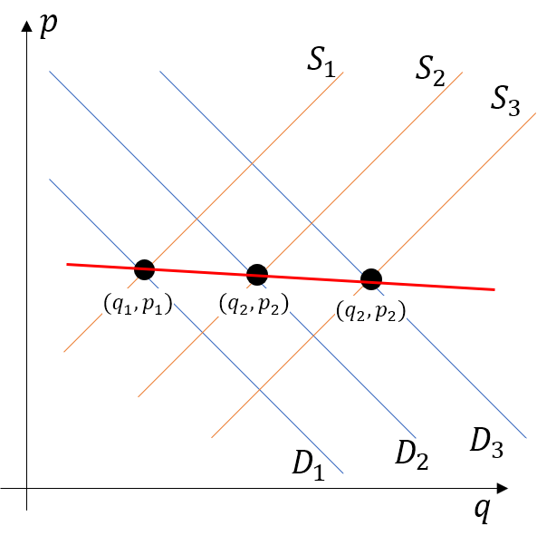
- Consider the demand and supply curve \[ \begin{aligned} q^{d} =\beta_{0}^{d}+\beta_{1}^{d}p+\beta_{2}^{d}x+u^{d} \\ q^{s} =\beta_{0}^{s}+\beta_{1}^{s}p+\beta_{2}^{s}z+u^{s} \end{aligned} \]
- The equilibrium price and quantity are determined by \(q^{d}=q^{s}\).
In this case, \[ p=\frac{(\beta_{2}^{s}z-\beta_{2}^{d}z)+(\beta_{0}^{s}-\beta_{0}^{d})+(u^{s}-u^{d})}{\beta_{1}^{d}-\beta_{1}^{s}} \] implying the correlation between the price and the error term.
- Putting this differently, the data points we observed is the intersection of these supply and demand curves.
How can we distinguish demand and supply?
12.3 Idea of IV Regression
- Let’s start with a simple case. \[ y_i = \beta_0 + \beta_1 x_i + \epsilon_i, \] and \(Cov(x_i, \epsilon_i) \neq 0\).
- Now, we consider another variable \(z_i\), which we call instrumental variable (IV).
- Instrumental variable \(z_i\) should satisfies the following two conditions:
- Independence: \(Cov(z_i, \epsilon_i) = 0\). No correlation between IV and error.
- Relevance: \(Cov(z_i, x_i) \neq 0\). There should be correlation between IV and endogenous variable \(x_i\).
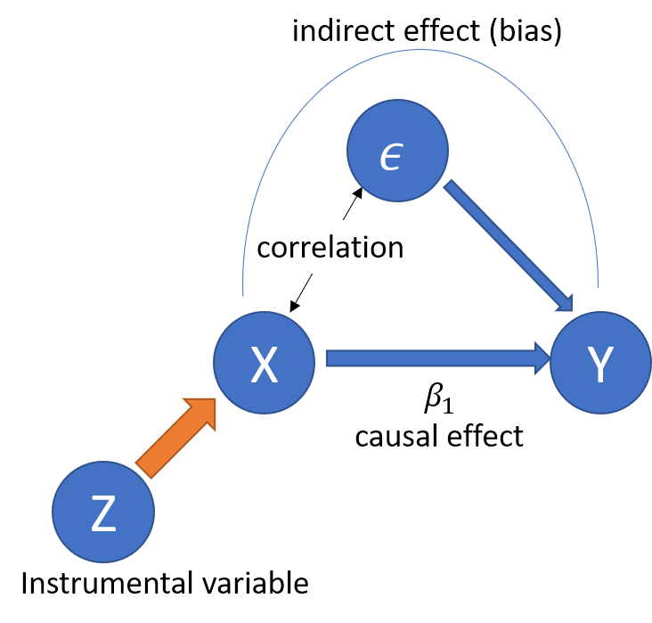
Idea: Use the variation of \(x_i\) induced by instrument \(z_i\) to estimate the direct (causal) effect of \(x_i\) on \(y_i\), that is \(\beta_1\)!.
- More on this:
- Intuitively, the OLS estimator captures the correlation between \(x\) and \(y\).
- If there is no correlation between \(x\) and \(\epsilon\), it captures the causal effect \(\beta_1\).
- If not, the OLS estimator captures both direct and indirect effect, the latter of which is bias.
- Now, let’s capture the variation of \(x\) due to instrument \(z\),
- Such a variation should exist under relevance assumption.
- Such a variation should not be correlated with the error under independence assumption
- By looking at the correlation between such variation and \(y\), you can get the causal effect \(\beta_1\).
Idea IV
12.4 Formal Framework and Estimation
12.4.1 Model
- We now introduce a general framework with multiple endogenous variables and multiple instruments.
- Consider the model \[
\begin{aligned}
Y_i = \beta_0 + \beta_1 X_{1i} + \dots + \beta_K X_{Ki} + \beta_{K+1} W_{1i} + \dots + \beta_{K+R} W_{Ri} + u_i,
\end{aligned}
\] with \(i=1,\dots,n\) is the general instrumental variables regression model where
- \(Y_i\) is the dependent variable
- \(\beta_0,\dots,\beta_{K+R}\) are \(1+K+R\) unknown regression coefficients
- \(X_{1i},\dots,X_{Ki}\) are \(K\) endogenous regressors: \(Cov(X_{ki}, u_i) \neq 0\) for all \(k\).
- \(W_{1i},\dots,W_{Ri}\) are \(R\) exogenous regressors which are uncorrelated with \(u_i\). \(Cov(W_{ri}, u_i) = 0\) for all \(r\).
- \(u_i\) is the error term
- \(Z_{1i},\dots,Z_{Mi}\) are \(M\) instrumental variables
- I will discuss conditions for valid instruments later.
12.4.2 Estimation by Two Stage Least Squares (2SLS)
- We can estimate the above model by Two Stage Least Squares (2SLS)
- Step 1: First-stage regression(s)
- Run an OLS regression for each of the endogenous variables (\(X_{1i},\dots,X_{ki}\)) on all instrumental variables (\(Z_{1i},\dots,Z_{mi}\)), all exogenous variables (\(W_{1i},\dots,W_{ri}\)) and an intercept.
- Compute the fitted values (\(\widehat{X}_{1i},\dots,\widehat{X}_{ki}\)).
- Step 2: Second-stage regression
- Regress the dependent variable \(Y_i\) on the predicted values of all endogenous regressors (\(\widehat{X}_{1i},\dots,\widehat{X}_{ki}\)), all exogenous variables (\(W_{1i},\dots,W_{ri}\)) and an intercept using OLS.
- This gives \(\widehat{\beta}_{0}^{TSLS},\dots,\widehat{\beta}_{k+r}^{TSLS}\), the 2SLS estimates of the model coefficients.
12.4.2.1 Intuition
- Why does this work? Let’s go back to the simple example with 1 endogenous variable and 1 IV.
- In the first stage, we estimate
\[ x_i = \pi_0 + \pi_1 z_i + v_i \] by OLS and obtain the fitted value \(\widehat{x}_i = \widehat{\pi}_0 + \widehat{\pi}_1 z_i\). - In the second stage, we estimate \[ y_i = \beta_0 + \beta_1 \widehat{x}_i + u_i \]
- Since \(\widehat{x}_i\) depends only on \(z_i\), which is uncorrelated with \(u_i\), the second stage can estimate \(\beta_1\) without bias.
- Can you see the importance of both independence and relevance asssumption here? (More formal discussion later)
12.4.3 Conditions for Valid IVs in a general framework
12.4.3.1 Necessary condition
- Depending on the number of IVs, we have three cases
- Over-identification: \(M > K\)
- Just identification] \(M=K\)
- Under-identification \(M < K\)
- The necessary condition is \(M \geq K\).
- We should have more IVs than endogenous variables!!
12.4.3.2 Sufficient condition
- How about sufficiency?
- In a general framework, the sufficient condition for valid instruments is given as follows.
- Independence: \(Cov( Z_{mi}, \epsilon_i) = 0\) for all \(m\).
- Relevance: In the second stage regression, the variables \[ \left( \widehat{X}_{1i},\dots,\widehat{X}_{ki}, W_{1i},\dots,W_{ri}, 1 \right) \] are not perfectly multicollinear.
- What does the relevance condition mean?
- In the simple example above, The first stage is
\[ x_i = \pi_0 + \pi_1 z_i + v_i \] and the second stage is \[ y_i = \beta_0 + \beta_1 \widehat{x}_i + u_i \] - The second stage would have perfect multicollinarity if \(\pi_1 = 0\) (i.e., \(\widehat{x}_i = \pi_0\)).
- Back to the general case, the first stage for \(X_k\) can be written as \[ X_{ki} = \pi_0 + \pi_1 Z_{1i} + \cdots + \pi_M Z_{Mi} + \pi_{M+1} W_{1i} + \cdots + \pi_{M+R} W_{Ri} \] and one of \(\pi_1 , \cdots, \pi_M\) should be non-zero.
- Intuitively speaking, the instruments should be correlated with endogenous variables after controlling for exogenous variables
12.5 Check Instrument Validity
12.5.1 Relevance
- Instruments are weak if those instruments explain little variation in the endogenous variables.
- Weak instruments lead to
- imprecise estimates (higher standard errors)
- The asymptotic distribution would deviate from a normal distribution even if we have a large sample.
- Here is a rule of thumb to check the relevance conditions.
- Consider the case with one endogenous variable \(X_{1i}\).
- The first stage regression
\[ X_k = \pi_0 + \pi_1 Z_{1i} + \cdots + \pi_M Z_{Mi} + \pi_{M+1} W_{1i} + \cdots + \pi_{M+R} W_{Ri} \] - And test the null hypothesis \[
\begin{aligned}
H_0 & : \pi_1 = \cdots = \pi_M = 0 \\
H_1 & : otherwise
\end{aligned}
\]
- This is F test (test of joint hypothesis)
- If we can reject this, we can say no concern for weak instruments.
- A rule of thumbs is that the F statistic should be larger than 10.
12.5.1 Independence (Instrument exogeneity)
- Arguing for independence is hard and a key in empirical analysis.
- Justification of this assumption depends on a context, institutional features, etc…
- We will see this through examples in the next chapter.