9 Linear Regression 2: Implementation in R
9.1 Implementation in R
9.1.1 Preliminary: packages
- We use the following packages:
AER:dplyr: data manipulationstargazer: output of regression results
# Install package if you have not done so
# install.packages("AER")
# install.packages("dplyr")
# install.packages("stargazer")
# install.packages("lmtest")

# load packages
library("AER")
## 要求されたパッケージ car をロード中です## 要求されたパッケージ carData をロード中です## 要求されたパッケージ lmtest をロード中です## 要求されたパッケージ zoo をロード中です##
## 次のパッケージを付け加えます: 'zoo'## 以下のオブジェクトは 'package:base' からマスクされています:
##
## as.Date, as.Date.numeric## 要求されたパッケージ sandwich をロード中です## 要求されたパッケージ survival をロード中ですlibrary("dplyr")##
## 次のパッケージを付け加えます: 'dplyr'## 以下のオブジェクトは 'package:car' からマスクされています:
##
## recode## 以下のオブジェクトは 'package:stats' からマスクされています:
##
## filter, lag## 以下のオブジェクトは 'package:base' からマスクされています:
##
## intersect, setdiff, setequal, unionlibrary("stargazer")##
## Please cite as:## Hlavac, Marek (2018). stargazer: Well-Formatted Regression and Summary Statistics Tables.## R package version 5.2.2. https://CRAN.R-project.org/package=stargazerlibrary("lmtest")9.1.2 Empirical setting: Data from California School
- Question: How does the student-teacher ratio affects test scores?
- We use data from California school, which is included in
AERpackage.- See here for the details: https://www.rdocumentation.org/packages/AER/versions/1.2-6/topics/CASchools
# load the the data set in the workspace
data(CASchools)- Use
class()function to seeCASchoolsisdata.frameobject.
class(CASchools)## [1] "data.frame"- We take 2 steps for the analysis.
- Step 1: Look at data (descriptive analysis)
- Step 2: Run regression
9.1.3 Step 1: Descriptive analysis
- It is always important to grasp your data before running regression.
head()function give you a first overview of the data.
head(CASchools)## district school county grades students
## 1 75119 Sunol Glen Unified Alameda KK-08 195
## 2 61499 Manzanita Elementary Butte KK-08 240
## 3 61549 Thermalito Union Elementary Butte KK-08 1550
## 4 61457 Golden Feather Union Elementary Butte KK-08 243
## 5 61523 Palermo Union Elementary Butte KK-08 1335
## 6 62042 Burrel Union Elementary Fresno KK-08 137
## teachers calworks lunch computer expenditure income english read
## 1 10.90 0.5102 2.0408 67 6384.911 22.690001 0.000000 691.6
## 2 11.15 15.4167 47.9167 101 5099.381 9.824000 4.583333 660.5
## 3 82.90 55.0323 76.3226 169 5501.955 8.978000 30.000002 636.3
## 4 14.00 36.4754 77.0492 85 7101.831 8.978000 0.000000 651.9
## 5 71.50 33.1086 78.4270 171 5235.988 9.080333 13.857677 641.8
## 6 6.40 12.3188 86.9565 25 5580.147 10.415000 12.408759 605.7
## math
## 1 690.0
## 2 661.9
## 3 650.9
## 4 643.5
## 5 639.9
## 6 605.4- Alternatively, you can use
browse()to see the entire dataset in browser window.
9.1.3.1 Create variables
- Create several variables that are needed for the analysis.
- We use
dplyrfor this purpose.
CASchools %>%
  mutate( STR = students / teachers ) %>%
  mutate( score = (read + math) / 2 ) -> CASchools
9.1.3.2 Descriptive statistics
- There are several ways to show descriptive statistics
- The standard one is to use
summary()function
summary(CASchools)## district school county grades
## Length:420 Length:420 Sonoma : 29 KK-06: 61
## Class :character Class :character Kern : 27 KK-08:359
## Mode :character Mode :character Los Angeles: 27
## Tulare : 24
## San Diego : 21
## Santa Clara: 20
## (Other) :272
## students teachers calworks lunch
## Min. : 81.0 Min. : 4.85 Min. : 0.000 Min. : 0.00
## 1st Qu.: 379.0 1st Qu.: 19.66 1st Qu.: 4.395 1st Qu.: 23.28
## Median : 950.5 Median : 48.56 Median :10.520 Median : 41.75
## Mean : 2628.8 Mean : 129.07 Mean :13.246 Mean : 44.71
## 3rd Qu.: 3008.0 3rd Qu.: 146.35 3rd Qu.:18.981 3rd Qu.: 66.86
## Max. :27176.0 Max. :1429.00 Max. :78.994 Max. :100.00
##
## computer expenditure income english
## Min. : 0.0 Min. :3926 Min. : 5.335 Min. : 0.000
## 1st Qu.: 46.0 1st Qu.:4906 1st Qu.:10.639 1st Qu.: 1.941
## Median : 117.5 Median :5215 Median :13.728 Median : 8.778
## Mean : 303.4 Mean :5312 Mean :15.317 Mean :15.768
## 3rd Qu.: 375.2 3rd Qu.:5601 3rd Qu.:17.629 3rd Qu.:22.970
## Max. :3324.0 Max. :7712 Max. :55.328 Max. :85.540
##
## read math STR score
## Min. :604.5 Min. :605.4 Min. :14.00 Min. :605.5
## 1st Qu.:640.4 1st Qu.:639.4 1st Qu.:18.58 1st Qu.:640.0
## Median :655.8 Median :652.5 Median :19.72 Median :654.5
## Mean :655.0 Mean :653.3 Mean :19.64 Mean :654.2
## 3rd Qu.:668.7 3rd Qu.:665.9 3rd Qu.:20.87 3rd Qu.:666.7
## Max. :704.0 Max. :709.5 Max. :25.80 Max. :706.8
## - This returns the desriptive statistics for all the variables in dataframe.
- You can combine this with
dplyr::select
CASchools %>%
  select(STR, score) %>%
  summary()
## STR score
## Min. :14.00 Min. :605.5
## 1st Qu.:18.58 1st Qu.:640.0
## Median :19.72 Median :654.5
## Mean :19.64 Mean :654.2
## 3rd Qu.:20.87 3rd Qu.:666.7
## Max. :25.80 Max. :706.8- You can do a bit lengthly thing manually like this.
# compute sample averages of STR and score
avg_STR <- mean(CASchools$STR)
avg_score <- mean(CASchools$score)

# compute sample standard deviations of STR and score
sd_STR <- sd(CASchools$STR)
sd_score <- sd(CASchools$score)

# set up a vector of percentiles and compute the quantiles
quantiles <- c(0.10, 0.25, 0.4, 0.5, 0.6, 0.75, 0.9)
quant_STR <- quantile(CASchools$STR, quantiles)
quant_score <- quantile(CASchools$score, quantiles)

# gather everything in a data.frame
DistributionSummary <- data.frame(Average = c(avg_STR, avg_score),
                                  StandardDeviation = c(sd_STR, sd_score),
                                  quantile = rbind(quant_STR, quant_score))

# print the summary to the console
DistributionSummary
## Average StandardDeviation quantile.10. quantile.25.
## quant_STR 19.64043 1.891812 17.3486 18.58236
## quant_score 654.15655 19.053347 630.3950 640.05000
## quantile.40. quantile.50. quantile.60. quantile.75.
## quant_STR 19.26618 19.72321 20.0783 20.87181
## quant_score 649.06999 654.45000 659.4000 666.66249
## quantile.90.
## quant_STR 21.86741
## quant_score 678.85999- My personal favorite is to use
stargazerfunction.
stargazer(CASchools, type = "text")##
## ===========================================================================
## Statistic N Mean St. Dev. Min Pctl(25) Pctl(75) Max
## ---------------------------------------------------------------------------
## students 420 2,628.793 3,913.105 81 379 3,008 27,176
## teachers 420 129.067 187.913 4.850 19.662 146.350 1,429.000
## calworks 420 13.246 11.455 0.000 4.395 18.981 78.994
## lunch 420 44.705 27.123 0.000 23.282 66.865 100.000
## computer 420 303.383 441.341 0 46 375.2 3,324
## expenditure 420 5,312.408 633.937 3,926.070 4,906.180 5,601.401 7,711.507
## income 420 15.317 7.226 5.335 10.639 17.629 55.328
## english 420 15.768 18.286 0 1.9 23.0 86
## read 420 654.970 20.108 604.500 640.400 668.725 704.000
## math 420 653.343 18.754 605 639.4 665.8 710
## STR 420 19.640 1.892 14.000 18.582 20.872 25.800
## score 420 654.157 19.053 605.550 640.050 666.662 706.750
## ---------------------------------------------------------------------------- You can choose summary statistics you want to report.
CASchools %>%
  stargazer( type = "text", summary.stat = c("n", "p75", "sd") )
##
## ===================================
## Statistic N Pctl(75) St. Dev.
## -----------------------------------
## students 420 3,008 3,913.105
## teachers 420 146.350 187.913
## calworks 420 18.981 11.455
## lunch 420 66.865 27.123
## computer 420 375.2 441.341
## expenditure 420 5,601.401 633.937
## income 420 17.629 7.226
## english 420 23.0 18.286
## read 420 668.725 20.108
## math 420 665.8 18.754
## STR 420 20.872 1.892
## score 420 666.662 19.053
## ------------------------------------ See https://www.jakeruss.com/cheatsheets/stargazer/#the-default-summary-statistics-table for the details.
- We will use
stargazerto report regression results.
9.1.3.3 Scatter plot
- Let’s see how test score and student-teacher-ratio is correlated.
plot(score ~ STR,
     data = CASchools,
     main = "Scatterplot of TestScore and STR",
     xlab = "STR (X)",
     ylab = "Test Score (Y)")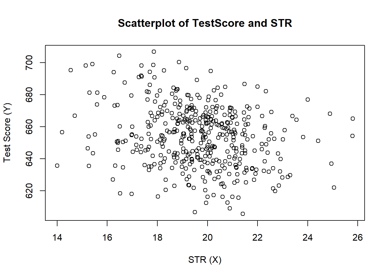
- Use
cor()to compute the correlation between two numeric vectors.
cor(CASchools$STR, CASchools$score)## [1] -0.22636279.1.4 Step 2: Run regression
9.1.4.1 Simple linear regression
- We use
lm()function to run linear regression - First, consider the simple linear regression \[
score_i = \beta_0 + \beta_1 size_i + \epsilon_i
\] where \(size_i\) is the class size (student-teacher-ratio).
- From now on we call student-teacher-ratio (STR) class size.
- To run this regression, we use
lm
# First, we rename the variable `STR`
CASchools %>%
  dplyr::rename( size = STR) -> CASchools

# Run regression and save results in the varaiable `model1_summary`
model1_summary <- lm( score ~ size, data = CASchools)

# See the results
summary(model1_summary)
##
## Call:
## lm(formula = score ~ size, data = CASchools)
##
## Residuals:
## Min 1Q Median 3Q Max
## -47.727 -14.251 0.483 12.822 48.540
##
## Coefficients:
## Estimate Std. Error t value Pr(>|t|)
## (Intercept) 698.9329 9.4675 73.825 < 0.0000000000000002 ***
## size -2.2798 0.4798 -4.751 0.00000278 ***
## ---
## Signif. codes: 0 '***' 0.001 '**' 0.01 '*' 0.05 '.' 0.1 ' ' 1
##
## Residual standard error: 18.58 on 418 degrees of freedom
## Multiple R-squared: 0.05124, Adjusted R-squared: 0.04897
## F-statistic: 22.58 on 1 and 418 DF, p-value: 0.000002783- Interpretations
- An increase of one student per teacher leads to 2.2 point decrease in test scores.
- p value is very small. The effect of the class size on test score is significant. Note: Be careful. These standard errors are NOT heteroskedasiticity robust. We will come back to this point soon.
- \(R^2 = 0.051\), implying that 5.1% of the variance of the dependent variable is explained by the model.
- You can add more variable in the regression (will see this soon)
9.1.4.2 Correction of Robust standard error
- We use
vcovHC()function, a partof the packagesandwich, to obtain the robust standard errors.- The package
sandwichis automatically loaded if you loadAERpackage.
- The package
# compute heteroskedasticity-robust standard errors
vcov <- vcovHC(model1_summary, type = "HC1")

# get standard error: the square root of the diagonal element in vcov
robust_se <- sqrt(diag(vcov))
robust_se
## (Intercept) size
## 10.3643617 0.5194893- Notice that robust standard errors are larger than the one we obtained from
lm! - How to combine the robust standard errors with the original summary? Use
coeftest()from the packagelmtest
# load `lmtest`
library(lmtest)

# Combine robust standard errors
coeftest(model1_summary, vcov. = vcov)
##
## t test of coefficients:
##
## Estimate Std. Error t value Pr(>|t|)
## (Intercept) 698.93295 10.36436 67.4362 < 0.00000000000000022 ***
## size -2.27981 0.51949 -4.3886 0.00001447 ***
## ---
## Signif. codes: 0 '***' 0.001 '**' 0.01 '*' 0.05 '.' 0.1 ' ' 19.1.4.3 Report by Stargazer
stargazeris useful to show the regression result.
# load
library(stargazer)

# Create output by stargazer
stargazer::stargazer(model1_summary, type ="text")
##
## ===============================================
## Dependent variable:
## ---------------------------
## score
## -----------------------------------------------
## size -2.280***
## (0.480)
##
## Constant 698.933***
## (9.467)
##
## -----------------------------------------------
## Observations 420
## R2 0.051
## Adjusted R2 0.049
## Residual Std. Error 18.581 (df = 418)
## F Statistic 22.575*** (df = 1; 418)
## ===============================================
## Note: *p<0.1; **p<0.05; ***p<0.01- Use robust standard errors in stargazer output
# Prepare robust standard errors in list
rob_se <- list( sqrt(diag(vcovHC(model1_summary, type = "HC1") ) ) )

# generate regression table.

stargazer( model1_summary,
           se = rob_se,
           type = "text")
##
## ===============================================
## Dependent variable:
## ---------------------------
## score
## -----------------------------------------------
## size -2.280***
## (0.519)
##
## Constant 698.933***
## (10.364)
##
## -----------------------------------------------
## Observations 420
## R2 0.051
## Adjusted R2 0.049
## Residual Std. Error 18.581 (df = 418)
## F Statistic 22.575*** (df = 1; 418)
## ===============================================
## Note: *p<0.1; **p<0.05; ***p<0.019.1.4.4 Full results
Taken from https://www.econometrics-with-r.org/7-6-analysis-of-the-test-score-data-set.html
# load the stargazer library

# estimate different model specifications
spec1 <- lm(score ~ size, data = CASchools)
spec2 <- lm(score ~ size + english, data = CASchools)
spec3 <- lm(score ~ size + english + lunch, data = CASchools)
spec4 <- lm(score ~ size + english + calworks, data = CASchools)
spec5 <- lm(score ~ size + english + lunch + calworks, data = CASchools)

# gather robust standard errors in a listh
rob_se <- list(sqrt(diag(vcovHC(spec1, type = "HC1"))),
               sqrt(diag(vcovHC(spec2, type = "HC1"))),
               sqrt(diag(vcovHC(spec3, type = "HC1"))),
               sqrt(diag(vcovHC(spec4, type = "HC1"))),
               sqrt(diag(vcovHC(spec5, type = "HC1"))))

# generate a LaTeX table using stargazer
stargazer(spec1, spec2, spec3, spec4, spec5,
          se = rob_se,
          digits = 3,
          header = F,
          column.labels = c("(I)", "(II)", "(III)", "(IV)", "(V)"),
          type ="text",
          keep.stat = c("N", "adj.rsq"))
##
## ===================================================================
## Dependent variable:
## ------------------------------------------------------
## score
## (I) (II) (III) (IV) (V)
## (1) (2) (3) (4) (5)
## -------------------------------------------------------------------
## size -2.280*** -1.101** -0.998*** -1.308*** -1.014***
## (0.519) (0.433) (0.270) (0.339) (0.269)
##
## english -0.650*** -0.122*** -0.488*** -0.130***
## (0.031) (0.033) (0.030) (0.036)
##
## lunch -0.547*** -0.529***
## (0.024) (0.038)
##
## calworks -0.790*** -0.048
## (0.068) (0.059)
##
## Constant 698.933*** 686.032*** 700.150*** 697.999*** 700.392***
## (10.364) (8.728) (5.568) (6.920) (5.537)
##
## -------------------------------------------------------------------
## Observations 420 420 420 420 420
## Adjusted R2 0.049 0.424 0.773 0.626 0.773
## ===================================================================
## Note: *p<0.1; **p<0.05; ***p<0.01- The coefficient on the class size decreases as we add more explantory variables. Can you explain why? (Hint: omitted variable bias)